Mean-Field Theories for Electronic Order
Mean-field theory replaces an interacting fermion Hamiltonian by a quadratic (Gaussian) variational Hamiltonian whose parameters are fixed by self-consistency:
The quadratic problem can be solved exactly (diagonalised), and all required expectation values are computed within that Gaussian reference state.
For superconducting order this is the standard route from BCS and Gor’kov mean-field theory to the BdG equations and their de Gennes real-space formulation, while in lattice-model language the same closure yields Hartree, Fock, and pairing channels for Hubbard-type and multiorbital interactions. [1, 2, 3, 4, 5, 6]
Throughout we keep the fixed tensor-product bookkeeping
where (\mathcal H_{\mathrm{int}}=\mathrm{span}{|m\rangle : m\in\mathscr M}) denotes the internal or orbital one-body space.
We therefore present each object first in compact tensor notation and then in explicit indices, consistent with the symmetry/tensor construction of the preceding chapters.
Conventions, dictionary, and Kronecker bookkeeping
This section fixes once-and-for-all the translation between explicit indices and operator/tensor (Kronecker) notation.
One-body space and composite indices
Let the physical (non-Nambu) one-body space be
and introduce a composite index
Collect annihilation operators into a column vector (\hat c) over (\mathcal H_1),
The equal-time correlators needed for self-consistency are then
In operator language, (ρ) and (χ) are matrices on (\mathcal H_1), i.e. (ρ,χ\in \mathrm{End}(\mathcal H_1)).
Kronecker placement and “who acts where”
If (A) acts on (\mathcal H_{\mathrm{lat}}) and (B) on (\mathcal H_{\mathrm{spin}}), then
acts on (\mathcal H_{\mathrm{lat}}\otimes\mathcal H_{\mathrm{spin}}), with the remaining factors understood to carry identities.
We will write identity operators as (𝟙_{\mathrm{lat}}), (𝟙_{\mathrm{Nambu}}), etc., and use a Pauli basis ({τ_\ell}) on Nambu space and ({σ_j}) on spin space:
It is also convenient to define raising/lowering combinations
so that Nambu block matrices can be written compactly as sums of Kronecker products.
Transpose, swap, and antisymmetry
In real-space/orbital/spin indices, the transpose (T) means swapping the composite indices:
Equivalently, introduce the swap operator (𝒫) on (\mathcal H_1\otimes\mathcal H_1) defined by
Then “antisymmetry under exchange” is expressed by the antisymmetriser (𝒜=(𝟙-𝒫)/2). In particular, fermionic antisymmetry of the pairing channel will be written as
i.e. (𝒫) projects out symmetric components in the combined indices.
Quadratic mean-field Hamiltonian: tensor form and explicit indices
Nambu spinor and BdG form
Introduce the Nambu spinor on the doubled one-body space (\mathcal H_{\mathrm{Nambu}}\otimes\mathcal H_1),
Then any quadratic BdG mean-field Hamiltonian can be written as
where (\boldsymbol{\mathcal H}^{\mathrm{MF}}) is a Hermitian matrix acting on (\mathcal H_{\mathrm{lat}}\otimes\mathcal H_{\mathrm{Nambu}}\otimes\mathcal H_{\mathrm{int}}\otimes\mathcal H_{\mathrm{spin}}), and (\mathcal E_{\mathrm{gs}}) is the mean-field ground-state (double-counting) constant.
In Nambu block form,
where (\boldsymbolΣ) collects all normal self-energies (Hartree/Fock-like) and (\boldsymbolΔ) is the anomalous (pairing) mean field. This is the standard Gor’kov/de Gennes BdG structure written in the tensor conventions used throughout the thesis. [2, 3]
A compact Kronecker representation of this BdG structure is
where (\boldsymbol h^{\mathrm{MF}}) and (\boldsymbolΔ) act on (\mathcal H_1) and the (τ)-matrices act on (\mathcal H_{\mathrm{Nambu}}).
Tensor expansion compatible with the symmetry construction
To maintain continuity with the shift/tensor template, expand (\boldsymbol{\mathcal H}^{\mathrm{MF}}) in a basis on the internal/Nambu/spin factors, with lattice operators as coefficients:
where ({τ_\ell}) is a Pauli basis on (\mathcal H_{\mathrm{Nambu}}), ({λ_i}) is a Hermitian operator basis on (\mathcal H_{\mathrm{int}}), ({σ_j}) is a Pauli basis on (\mathcal H_{\mathrm{spin}}), and (\mathbb X_{\ell i j}) are operators on (\mathcal H_{\mathrm{lat}}) (typically built from masked shifts, projectors, or inhomogeneous geometry operators).
This viewpoint emphasises that the mean-field problem remains “quadratic plus symmetry constraints”: once a symmetry generator set is chosen, the allowed channels (τ_\ell\otimesλ_i\otimesσ_j) are constrained exactly as in the free-fermion construction, while the lattice coefficients (\mathbb X_{\ell i j}) are determined self-consistently.
Explicit-index interaction channels
In explicit indices, the most general quadratic mean-field interaction on an arbitrary lattice (Ω) can be written as
Here (\symbf ρ) is Hartree-like (density) renormalisation, (\symbf Φ) is Fock-like (exchange/hopping renormalisation), and (\symbf Δ) is Gor’kov-like pairing. These channels exhaust the Wick contractions of a two-body interaction into quadratic (Gaussian) fields.[^1] In model Hamiltonians this is precisely the decomposition used for on-site and extended Hubbard interactions, as well as for multiorbital Kanamori-type local interactions. [4, 5, 6]
It is sometimes useful to recognise these as kernels on (\mathcal H_1):
with the precise identification fixed by the chosen microscopic interaction tensor (\symbf U) and by the “diagonal vs off-diagonal” decomposition in the chosen basis.
Variational free energy and mean-field stationarity
Mean-field free-energy decomposition
For the full interacting Hamiltonian (\hat{\mathcal H}=\hat{\mathcal H}_0+\hat{\mathcal H}I), the exact free energy is Mean-field theory approximates this by evaluating the expectation values in the Gaussian (quadratic) reference ensemble generated by (\hat{\mathcal H}^{\mathrm{MF}}{\mathrm{BdG}}):
Writing
one obtains the standard decomposition
Stationarity (saddle-point) of (F) with respect to the variational fields yields the self-consistency equations.[^2]
Stationarity as a restricted variational principle
Conceptually, mean-field theory minimises the exact free-energy functional over the restricted family of Gaussian density matrices:
This restriction is precisely what makes Wick factorisation exact inside the trial ensemble, and what turns the interacting problem into a closed fixed-point problem for the quadratic kernels (Σ) and (Δ). In the superconducting context this restricted variational logic is the standard mean-field closure behind BdG theory. [1, 3]
Wick reduction of (\langle \hat{\mathcal H}I\rangle{\mathrm{MF}})
For a density–density interaction (schematically (\hat{\mathcal H}_I=\sum U,\hat n\hat n)), Wick’s theorem gives, in explicit indices,
The exchange minus sign is enforced by fermionic anticommutation.
In composite-index language, a typical (model-dependent) rewriting is
where (U_{\alpha\beta}) is the interaction kernel in the (|\alpha\rangle) basis (site/orbital/spin).
To evaluate these expectation values systematically we introduce Matsubara kernels (imaginary-frequency resolvent kernels), rather than real-frequency Green’s functions.
Matsubara kernels for BdG mean-field theory
Imaginary-time kernel and Matsubara transform
Define the imaginary-time Nambu kernel
where (\hatΦ(τ)=e^{τ \hat{\mathcal H}^{\mathrm{MF}}{\mathrm{BdG}}}\hatΦ e^{-τ \hat{\mathcal H}^{\mathrm{MF}}{\mathrm{BdG}}}) and (\mathsf T_τ) is imaginary-time ordering.
The fermionic Matsubara components are
For a quadratic mean-field Hamiltonian, the kernel is the matrix inverse (imaginary-frequency resolvent)
This is the Matsubara analogue of the resolvent: it is the unique object from which all bilinear correlators follow by frequency summation (or integration at (T=0)). This is just the imaginary-frequency Green-function formulation of the same BdG mean-field problem. [2, 3]
Spectral expansion in the BdG eigenbasis
Let (\boldsymbol{\mathcal H}^{\mathrm{MF}}Ψ_r=\mathcal E_rΨ_r). The intrinsic BdG particle–hole symmetry implies a paired spectrum (\pm \mathcal E_r). The resolvent kernel has the spectral representation
where (\barΨ_r) is the particle–hole conjugate of (Ψ_r) (defined precisely below).
Normal/anomalous blocks and explicit-index kernels
Write the Nambu kernel in block form
where (\mathcal K) is the normal (particle–particle) kernel and (\mathcal L) is the anomalous (pairing) kernel. In Kronecker language, this block structure corresponds to the decomposition in (τ)-space.
In explicit indices (site (\mathbf i,\mathbf i’), spin (σ,σ’), orbitals (m,m’)), write (Ψ_r=((u_{\mathbf iσ m})r,(v{\mathbf iσ m})_r)). Then
and
Define the transpose in the combined non-Nambu indices by
Intrinsic BdG particle–hole symmetry implies the block relations
so that
Densities from Matsubara kernels
Equal-time correlators as Matsubara sums
For self-consistency we require normal and anomalous equal-time correlators:
These follow from the Matsubara kernels by
and in explicit indices,
Carrying out the Matsubara sums using the spectral representation yields the familiar BdG-eigenvector formulas at finite temperature:
Zero-temperature limit ((T\to0)): imaginary-frequency integrals and projectors
At finite temperature the Matsubara frequencies are discrete,
In the zero-temperature limit (β\to\infty), Matsubara sums become imaginary-frequency integrals:
so one may compute observables directly from (\boldsymbol{\mathcal K}(iω)) without analytic continuation to real frequency.
Equivalently (and most usefully in BdG numerics), equal-time correlators become projectors onto the occupied (negative-energy) BdG subspace. Define the occupied projector
In Nambu block form this projector has the universal structure
where the transpose is taken in the combined non-Nambu indices. Thus (ρ) and (χ) may be obtained either from the imaginary-frequency integral formula above or directly from (𝒫_-). In explicit indices (including negative-energy eigenvectors),
which is precisely the (T\to0) limit of the finite-(T) Fermi-factor formulas, (f(\mathcal E)\to Θ(-\mathcal E)).
Self-consistency equations: tensor/Kronecker form and explicit indices
The variational stationarity condition (\delta F=0) yields
The resulting saddle-point equations can be expressed compactly as “interaction tensor (\times) densities”.
Compact tensor form (channel superoperators)
Write the microscopic interaction kernel as a tensor (U) in the composite basis,
Introduce the diagonal-extraction superoperator (𝒟) (in the chosen local basis) defined by
and recall that matrix transpose is ((A^T){\alpha\beta}=A{\beta\alpha}).
Then the three mean-field channels may be represented schematically as
with the understanding that “(U)” here denotes the appropriate contraction of interaction indices with the density matrices in the same basis used to define (U_{\alpha\beta}). This tensor form makes the physics transparent: Hartree couples to the diagonal density, Fock to exchange (transpose), and pairing to the anomalous correlator.
The intrinsic fermionic antisymmetry constraint (independent of TRS) is
i.e. only antisymmetric components in combined indices contribute to pairing.
Explicit-index form (matching your notation)
In explicit-index form (as used throughout your construction),
The symmetry (\symbf{U}{\mathbf{i},\mathbf{j},σ,τ,m,n}= \symbf{U}{\mathbf{j},\mathbf{i},τ,σ,n,m}), together with fermionic algebra, implies in common gauges
The resulting mean-field Hamiltonian is therefore
Homogeneous bulk BCS benchmarks
Before turning to spatially inhomogeneous textures, it is useful to examine the same self-consistency equations in uniform bulk settings. Even in this simplest limit, the fixed-point problem already shows the characteristic separation between weak, intermediate, and strong coupling, together with a strong dependence on the underlying normal-state density of states. This is the usual BCS-to-strong-coupling mean-field phenomenology for attractive lattice models. [1, 5]
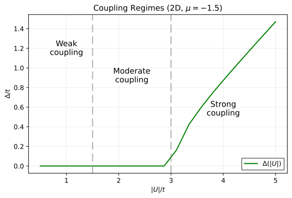
Illustrative two-dimensional bulk BCS benchmark showing the self-consistent zero-temperature gap as a function of interaction strength for chemical potential . The weak-coupling regime is exponentially suppressed, the intermediate regime marks the rapid onset of pairing, and the strong-coupling regime crosses over toward large local pair formation.
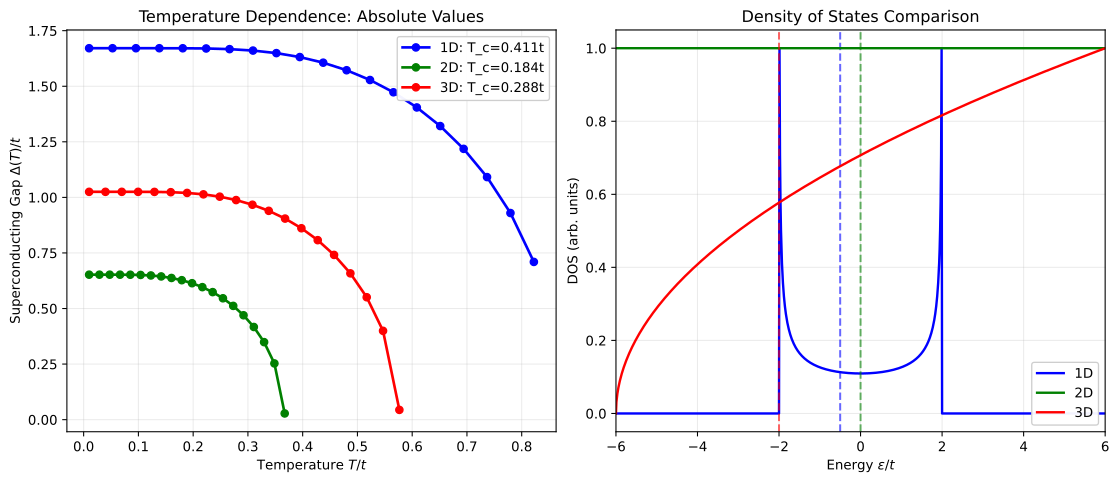
Bulk BCS temperature and density-of-states comparison for simple one-, two-, and three-dimensional model dispersions. The left panel shows the self-consistent gap decreasing toward the critical temperature in each dimension, while the right panel shows how differences in the normal-state density of states help set the pairing scale and the most favorable chemical-potential window.
Gaussian fluctuations about the mean-field saddle
Mean-field theory corresponds to a saddle point of the variational free-energy functional restricted to Gaussian density matrices. To go beyond static mean-field theory, we expand the free energy to quadratic order in fluctuations of the mean fields. This yields a controlled description of collective modes (RPA, Anderson–Bogoliubov, amplitude modes, etc.) and provides the starting point for diagrammatic and numerical extensions. In superconductors this is the standard route from static BdG mean field to RPA/Gaussian collective-mode theory. [7, 8, 3]
Throughout this section, all indices and tensor placements follow the conventions fixed above.
Fluctuating fields and parametrisation
Write the BdG kernel as a saddle-point value plus fluctuations:
In Nambu block form,
where
represent fluctuations in the normal and anomalous channels.
In composite-index notation,
We group all fluctuating fields into a single vector:
with the understanding that symmetry constraints (Hermiticity, antisymmetry) are enforced either explicitly or by restricting the independent components.
Expansion of the free energy
The mean-field free energy may be written as
where the trace includes Matsubara frequency, Nambu space, and (\mathcal H_1).
Expanding to second order about the saddle point,
First variation (vanishes at self-consistency)
The linear term is
where
Using the saddle-point equations derived above, one has
which is simply the statement that mean-field theory is stationary.
Second variation: general structure
The quadratic fluctuation action is
This has a universal structure:
where (\mathcal M) is the Gaussian fluctuation kernel (inverse propagator of collective modes).
Explicit evaluation of the fermionic loop
Write the trace explicitly:
Separating normal and anomalous parts gives three types of contributions:
(i) Density—density (normal—normal)
(ii) Pairing—pairing
(iii) Mixed normal—anomalous
These expressions are exact for Gaussian fluctuations.
Interaction contribution and RPA structure
The interaction part contributes a local quadratic form:
with
Combining fermionic loops and interaction terms yields the standard RPA / Gaussian-fluctuation kernel
where (\Pi) is the generalized susceptibility matrix constructed from two BdG propagators. This is the superconducting analogue of the usual RPA inverse propagator, now written in Nambu-channel form. [7]
Explicit susceptibility tensor (ready for coding)
Define a collective-channel index (A=(\alpha\beta,\mu)) with
Then
where the vertex matrices are
At zero external frequency ((Ω_m=0)), this kernel controls static stability; its zeros correspond to Goldstone modes and instabilities.
Physical content
- Positive-definiteness of (\mathcal M) ⇔ local stability of the mean-field saddle.
- Zero eigenvalues ⇔ spontaneous symmetry breaking (phase mode).
- Poles of (\mathcal M^{-1}(iΩ)) ⇔ collective excitations.
- Restricting to the pairing sector reproduces the standard BCS amplitude/phase fluctuation theory.
- Keeping full index structure allows spatially inhomogeneous and multiorbital collective modes.
In the superconducting case this reproduces the familiar Anderson-Bogoliubov phase mode and its gauge-coupled descendants. [7, 8]
Minimal numerical recipe
- Solve BdG → obtain (\boldsymbol{\mathcal K}(iω_n)).
- Build (\Pi) via Matsubara sums of kernel products.
- Form (\mathcal M = U^{-1}-\Pi).
- Diagonalise (\mathcal M) (static) or (\mathcal M(iΩ)) (dynamic).
- Interpret eigenvectors in composite-index space.
This formulation is directly compatible with sparse real-space BdG codes and symmetry-restricted tensor constructions.
BdG eigenproblem and quasiparticles
Solve the BdG eigenproblem
with components (u_r={(u_{\mathbf iσ m})r}) and (v_r={(v{\mathbf iσ m})_r}). The corresponding Bogoliubov quasiparticles (\hatγ_r) diagonalise the quadratic Hamiltonian:
with the (\pm\mathcal E_r) pairing enforced by intrinsic BdG particle–hole symmetry. This is the standard Bogoliubov quasiparticle construction in the de Gennes formulation. [3]
Time-reversal symmetry (TRS) and intrinsic BdG particle—hole symmetry (PHS)
This section treats time-reversal symmetry (TRS) as an optional physical symmetry constraint on (\boldsymbol{\mathcal H}^{\mathrm{MF}}), and particle–hole symmetry (PHS) as an intrinsic constraint of the BdG/Nambu representation.
TRS: definition and BdG constraint (operator and tensor form)
Let (\hat{\mathcal C}) denote complex conjugation in the chosen basis. For spin-(\tfrac12) electrons define the antiunitary time-reversal operator on (\mathcal H_1),
In real space,
and in translation-invariant systems TRS flips momentum (\mathbf k\mapsto -\mathbf k).
On BdG/Nambu space, take the induced unitary part acting diagonally in particle/hole components:
TRS of the BdG mean-field Hamiltonian is then the conjugation constraint
In Nambu blocks this implies
where (U_{\mathsf T}=𝟙_{\mathrm{lat}}\otimes 𝟙_{\mathrm{int}}\otimes(-iσ_y)) acts on the non-Nambu factors.
TRS as a constraint on tensor/Kronecker channels
Using the expansion
TRS becomes a selection rule on allowed channels:
and the lattice operators (\mathbb X_{\ell i j}) must satisfy the corresponding relations (including (\mathbf k\mapsto -\mathbf k) if applicable). In practice this is the cleanest way to enforce TRS while building a symmetry-adapted mean-field ansatz. This is also the natural language used in symmetry classifications of unconventional superconducting order parameters. [9]
Intrinsic BdG PHS: definition, spectrum pairing, and pairing antisymmetry
BdG Hamiltonians possess an intrinsic antiunitary particle–hole symmetry because the Nambu basis is redundant. Define
with unitary part (U_{\mathsf C}=𝟙_{\mathrm{lat}}\otimes τ_x\otimes 𝟙_{\mathrm{int}}\otimes 𝟙_{\mathrm{spin}}). The intrinsic BdG constraint is
Consequently, if (\boldsymbol{\mathcal H}^{\mathrm{MF}}Ψ=EΨ), then (\barΨ:=U_{\mathsf C}Ψ^) satisfies (\boldsymbol{\mathcal H}^{\mathrm{MF}}\barΨ=-E\barΨ), explaining the (\pm E) pairing of the BdG spectrum. In components, this corresponds to the familiar mapping ((u,v)\mapsto(-v^,u^*)) (up to Nambu convention).
Independently of TRS, fermionic antisymmetry imposes antisymmetry of the pairing kernel under exchange of combined indices:
In swap-operator language this is (𝒫,Δ,𝒫=-Δ), i.e. (Δ) lives in the antisymmetric sector selected by (𝒜).
Symmetry constraints on Matsubara kernels
Recall
From TRS one obtains
and from intrinsic BdG PHS,
These kernel constraints are the Matsubara-resolvent versions of the usual BdG symmetry relations and imply the block identities used above, such as (\bar{\mathcal K}(iω_n)=-\mathcal K(-iω_n)^{\mathrm T}) and (\bar{\mathcal L}(iω_n)=\mathcal L(iω_n)^\dagger).
Aside: Relation to DFT, Kohn—Sham, and SCDFT
Mean-field BdG theory and Kohn–Sham (KS) density-functional theory share a common structural theme—both solve a self-consistent quadratic problem—but differ in what is taken as fundamental and what is approximate.
Mean-field as a restricted variational principle
Mean-field theory may be viewed as a restricted variational problem: one minimises the exact free-energy functional over the subset of density matrices generated by quadratic trial Hamiltonians,
leading to saddle-point (self-consistency) equations for (Σ) and (Δ). The microscopic interaction tensor (\symbf U) explicitly determines which channels appear and how they couple.
DFT and Kohn—Sham: a universal functional and an auxiliary quadratic system
Ground-state DFT asserts that the ground-state density determines the external potential (up to a constant), and that the ground-state energy may be written as a universal functional of the density [10]. The KS construction introduces a non-interacting auxiliary system that reproduces the interacting density [11]. In lattice language one may write schematically
with (v_{xc,\mathbf i}[n]=\delta \mathcal F_{xc}/\delta n_{\mathbf i}). Thus the form of the quadratic problem resembles Hartree-like self-consistency, but the interpretation is different: interactions are encoded in universal functionals rather than via decoupling a chosen microscopic (\symbf U).
Finite-temperature DFT (Mermin) and the mean-field free energy
Because the present derivation is explicitly at finite temperature, the closest DFT analogue is Mermin’s extension of DFT to thermal ensembles, formulated as a variational principle for the free energy [12]. This is the clean point of contact: both approaches are naturally expressed at the level of a thermodynamic potential and solved by self-consistent Euler–Lagrange equations, though the underlying functionals and approximations differ.
SCDFT: a Kohn—Sham—BdG structure
Superconducting DFT extends DFT by enlarging the basic variables to include an anomalous (pair) density (χ(\mathbf r,\mathbf r’)=\langle \hatψ_\downarrow(\mathbf r)\hatψ_\uparrow(\mathbf r’)\rangle), leading to KS-like equations with a BdG structure [13]. This gives a clean mathematical mapping to self-consistent BdG, but only at the level of the fixed-point equations. The two theories are not equivalent: their Nambu matrices can be written in the same form, but the entries are generated by different closures.
On the SCDFT side one solves a superconducting Kohn–Sham problem of the form
Here both the normal KS operator and the pairing field are functionals of the normal and anomalous densities. In continuum language one may write schematically
and the densities are reconstructed self-consistently from the quasiparticle amplitudes. This is the superconducting analogue of the KS construction: the quadratic auxiliary problem is chosen so as to reproduce the interacting densities, not because the electrons are assumed to interact only through a particular microscopic model tensor.
By contrast, the self-consistent BdG problem developed in this chapter starts from a chosen low-energy Hamiltonian and a chosen interaction tensor (\symbf U). After mean-field decoupling one obtains
with (ρ_{\alpha\beta}=\langle \hat c^\dagger_\beta \hat c_\alpha\rangle) and (χ_{\alpha\beta}=\langle \hat c_\beta \hat c_\alpha\rangle) exactly as in the rest of this chapter. In the simplest pairing-only closure this is just the usual gap equation (Δ\sim -U,χ), while Hartree and Fock corrections sit in (Σ_{\mathrm{MF}}[ρ]).
A basis-level dictionary
Once both theories are expanded in a finite localized basis, the algebraic correspondence is immediate:
Normal density maps to the Hartree/Fock density matrix, anomalous density maps to the pair amplitude, the KS pairing field maps to the BdG gap matrix, and the KS normal potential maps to the mean-field normal Hamiltonian. This is why a Wannier-basis KS-BdG calculation and a multiorbital lattice BdG calculation can look almost indistinguishable numerically even though they arise from different theories.
Where the mapping stops
The decisive difference is the origin of the self-consistency closure. In SCDFT, the pairing field arises in principle from an exchange-correlation functional derivative with respect to the anomalous density,
and the normal KS potential likewise comes from functional derivatives with respect to the normal density [13]. In model BdG, by contrast, the gap and self-energy come from the explicit decoupling of a chosen microscopic interaction tensor (\symbf U). One may therefore regard self-consistent BdG as a restricted KS-BdG-shaped fixed-point problem with a model closure, but not as SCDFT itself.
That distinction matters physically. A lattice BdG solver is an effective low-energy mean-field theory: it is excellent for testing candidate order parameters, symmetry constraints, multiband structure, or TRSB mechanisms inside a chosen model space. It does not automatically supply the material-specific exchange-correlation pairing kernel, retardation effects, screened Coulomb physics, or full density feedback that belong to a bona fide superconducting density-functional treatment. The mathematically honest statement is therefore that self-consistent BdG and KS-BdG share a common Nambu structure, while SCDFT differs in how the normal and anomalous fields are generated.
Completing the finite-basis functional derivation
The cleanest way to make the relation precise in the notation of this chapter is to write a finite-basis free-energy functional directly in terms of the normal and anomalous one-body densities,
Here (ρ) and (χ) are the density matrices already introduced above, while (\mathcal T_s) and (\mathcal S) are understood as the kinetic and entropic contributions of the quadratic auxiliary problem. Stationarity with respect to the Gaussian reference state then produces a KS-BdG-shaped Euler equation on the Nambu-doubled one-body space,
with
This is the finite-basis SCDFT statement relevant to the thesis: once the closure is supplied by a bona fide functional of (ρ) and (χ), the quadratic fixed-point problem solved by the code is already of KS-BdG type.
Model BdG is recovered as the special case in which one chooses a restricted approximate functional rather than a universal superconducting density functional. For example, if one writes
with a pairing contribution of the schematic form
then variation immediately gives a BdG-style closure
together with the corresponding normal self-energy from (\mathcal F_{\mathrm{normal}}^{\mathrm{model}}[ρ]). In that sense every self-consistent quadratic BdG theory can be embedded in an SCDFT-shaped variational structure; what changes from theory to theory is the choice of functional closure.
This is also the precise point at which the scope of the present codebase should be understood. Our generalized quadratic solver is already broad enough to host either kind of closure:
- a model closure of the form (Σ[ρ]), (Δ[χ]), giving ordinary self-consistent BdG;
- a functional closure of the form (V_{xc}[ρ,χ]), (Δ_{xc}[ρ,χ]), giving a finite-basis SCDFT-style implementation.
What it does not provide automatically is the microscopic construction of the superconducting exchange-correlation functional itself. That object still has to be supplied, approximated, or derived. So the code already contains the universal quadratic backend required by SCDFT, but SCDFT as a first-principles theory is only obtained once that functional layer is specified.
References
- J. Bardeen, L. Cooper, and J. Schrieffer,
Theory of superconductivity,
Phys. Rev., vol. 108, no. 5, pp. 1175–1204, 1957. doi:10.1103/PhysRev.108.1175 (↩︎) - L. Gor’kov,
Microscopic derivation of the ginzburg–landau equations in the theory of superconductivity,
Soviet Physics JETP, vol. 9, no. 6, pp. 1364–1367, 1959. (↩︎) - P. Gennes, Superconductivity of metals and alloys. Boca Raton: CRC Press, 2019. doi:10.1201/9780429497032 (↩︎)
- J. Hubbard,
Electron correlations in narrow energy bands,
Proceedings of the Royal Society of London. Series A. Mathematical and Physical Sciences, vol. 276, pp. 238–257, 1963. doi:10.1098/rspa.1963.0204 (↩︎) - R. Micnas, J. Ranninger, and S. Robaszkiewicz,
Superconductivity in narrow-band systems with local nonretarded attractive interactions,
Reviews of Modern Physics, vol. 62, pp. 113–171, 1990. doi:10.1103/revmodphys.62.113 (↩︎) - J. Kanamori,
Electron correlation and ferromagnetism of transition metals,
Progress of Theoretical Physics, vol. 30, pp. 275–289, 1963. doi:10.1143/ptp.30.275 (↩︎) - P. Anderson,
Random-phase approximation in the theory of superconductivity,
Physical Review, vol. 112, pp. 1900–1916, 1958. doi:10.1103/physrev.112.1900 (↩︎) - P. Anderson,
Plasmons, gauge invariance, and mass,
Physical Review, vol. 130, pp. 439–442, 1963. doi:10.1103/physrev.130.439 (↩︎) - M. Sigrist and K. Ueda,
Phenomenological theory of unconventional superconductivity,
Reviews of Modern Physics, vol. 63, pp. 239–311, 1991. doi:10.1103/revmodphys.63.239 (↩︎) - P. Hohenberg and W. Kohn,
Inhomogeneous electron gas,
Physical Review, vol. 136, pp. B864–B871, 1964. doi:10.1103/physrev.136.b864 (↩︎) - W. Kohn and L. Sham,
Self-consistent equations including exchange and correlation effects,
Physical Review, vol. 140, pp. A1133–A1138, 1965. doi:10.1103/physrev.140.a1133 (↩︎) - N. Mermin,
Thermal properties of the inhomogeneous electron gas,
Physical Review, vol. 137, pp. A1441–A1443, 1965. doi:10.1103/physrev.137.a1441 (↩︎) - L. Oliveira, E. Gross, and W. Kohn,
Density-functional theory for superconductors,
Physical Review Letters, vol. 60, pp. 2430–2433, 1988. doi:10.1103/physrevlett.60.2430 (↩︎)