Introduction
Quantum Tensor Tree is introduced here not as a tensor-network ansatz in the MPS or TTN sense, but as a modelling language for quantum matter with visible internal structure. The central problem is simple to state. In the systems studied in this thesis, the physically relevant degrees of freedom are rarely well described by one flat integer index. One must keep track of site, orbital, spin, Nambu sector, unit-cell position, finite geometry, and in some cases larger mesoscopic aggregates such as superconducting islands. If that structure is erased too early, the notation may become numerically convenient, but the physics becomes harder to read and harder to control.
The framework therefore begins from the methodological claim that hierarchical physical structure should remain explicit for as long as possible. One should be able to describe a model first in the language in which the physics is naturally stated, and only later translate that description into arrays and matrices for numerical work. In this sense Quantum Tensor Tree is less a specialised software trick than a commitment about how quantum models should be represented.
This choice matters directly for the thesis. Loop-supercurrent states depend on
phase structure inside a small composite object rather than only on a large
translation-invariant lattice. The SSH and Topo-BdG chapters depend on the
ability to talk cleanly about boundaries, masks, walls, and finite cutouts.
Self-consistent superconducting calculations depend on distinguishing geometry,
Hamiltonian terms, and field-update rules rather than mixing them into one
opaque solver script. The live implementation in qulab/core/qttree, together
with the superconducting layer in qulab/core/scmft, should therefore be read
as a layered framework for preserving physical meaning through those different
tasks.
The novelty of the framework should therefore be stated carefully. It is not primarily that a new numerical algorithm was invented, nor that a new software package was written in the abstract. The conceptual contribution is that the thesis adopts a different modelling stance: physical hierarchy is treated as a first-class object; compilation is treated as an explicit boundary rather than an invisible implementation detail; and finite, Bloch, topological, and self-consistent superconducting problems are treated as different uses of one common modelling language rather than as separate code lineages.
Quantum Tensor Tree
The current package is layered: labelled basis objects feed model objects, which are then compiled, solved, and observed.
The thesis code spine
The final codebase should be read as a spine rather than as a collection of
independent packages. Quantum Tensor Tree supplies the model language:
labelled degrees of freedom, graph and lattice support, Hamiltonian terms, and
the compilation boundary where readable physics becomes numerical arrays.
qulab.core.qttree owns that language. qulab.core.qtopology then owns the
topological interpretation of SSH and Weyl–SSH models. qulab.core.scmft owns
the superconducting interpretation of pairing fields, anomalous contractions,
self-consistent updates, and free-energy branch comparisons. Finally, the
research/result records connect package paths to the model, benchmark, plotting,
and chapter paths that reproduce each thesis result.
The search code used in the loop-supercurrent work is part of this same spine. It is not a separate optimisation project detached from the physics framework. The genetic algorithms live at the study layer: they call QTT and SCMFT model constructors, evaluate cheap susceptibility or anomalous-density diagnostics, and then hand a small number of promising points back to the full branch-comparison machinery. This is a useful example of the architecture because it separates representation, solver, observable, and search. QTT describes the family of devices; SCMFT evaluates the mean-field branches; the search routine proposes where to spend expensive solver time.
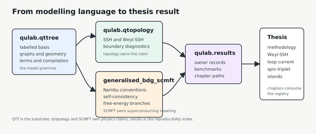
Figure 10.1: Package-level study spine from QTT through topology, SCMFT, result records, and thesis chapters.
This split is important because it prevents the code architecture from
overclaiming. QTT can describe the support of pairing-like terms and
current-carrying links, but it does not by itself decide what a superconducting
branch means. That decision requires Nambu conventions, anomalous density
updates, mean-field constants, and free-energy comparisons, which are the
responsibility of the generalised BdG/SCMFT layer. Likewise, a Weyl–SSH model
may use QTT constructors and may borrow SCMFT helpers for a paired extension,
but the central physical claim is topological and therefore belongs to
qulab.core.qtopology.
The four main studies in the thesis are therefore not four software lineages. They are four uses of one modelling framework:
- Weyl–SSH topology: a boundary and impurity-wall laboratory whose result narrative is topological.
- Microscopic loop-supercurrent: a self-consistent BdG/HFG test of whether a normal-spacer mechanism selects winding order.
- Spin-triplet TRSB: a multiorbital internally antisymmetric triplet test of channel selection, nonunitary diagnostics, and nonlinear limitations.
- Macroscopic islands: a controlled realisation layer for loop-supercurrent physics once the microscopic spacer mechanism is too weak or too costly.
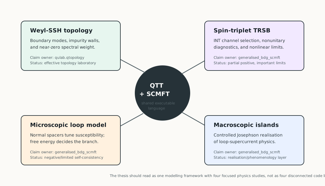
Figure 10.2: The four main thesis studies around the shared QTT and SCMFT infrastructure.
Relation to existing literatures
The ingredients of Quantum Tensor Tree are not individually new. Tight-binding and Bloch modelling already provide the standard language for lattice Hamiltonians and translationally invariant single-particle structure [1, 2]. Gor’kov, Bogoliubov-de Gennes, and de Gennes theory already provide the standard quadratic mean-field language for superconductivity [3, 4, 5]. Hubbard and Kanamori-type models already provide the standard interaction language for local and multiorbital electronic structure [6, 7, 8].
The methodological question is therefore not whether QTTree replaces those theories. It does not. The question is how one can express them inside one reusable modelling framework without fragmenting the thesis into separate code lineages for normal-state conductors, inhomogeneous superconductors, loop-supercurrent models, and boundary-sensitive topological problems. The novelty claimed here is architectural and methodological: one common modelling language preserves physical hierarchy, makes compilation into numerical form an explicit step, and terminates in a shared observable layer.
The closest external comparison is pyqula, which is impressively terse for
constructing and analysing tight-binding, superconducting, magnetic, and
topological models. That terseness is a useful standard: a thesis framework
should not require pages of boilerplate before a Hamiltonian can be inspected.
Where Quantum Tensor Tree differs is in what it chooses to make explicit. QTT
keeps labelled basis structure, support regions, symmetry sectors, interaction
channels, Nambu conventions, and free-energy accounting visible as named
objects. The aim is therefore not to be broader than pyqula, but to make the
particular modelling chain used in this thesis auditable from physical
declaration through compilation, self-consistency, observable extraction, and
figure reproduction.
This comparison also sets a practical convention for the codebase. Public examples should be terse at the point of use, but not by hiding physical choices that matter for the thesis. A good QTT example should read like a short model definition; its defaults should still leave a route back to the basis ordering, projector support, interaction channel, solver convention, and result provenance.
This chapter therefore has a deliberately limited scope. It is not an API
reference for every live module under qulab/core/qttree or
qulab/core/scmft, and it is not the right place to catalogue every helper,
benchmark wrapper, materials import path, or figure builder. Its purpose is to
explain the conceptual architecture that the thesis is claiming as method. A
separate code-facing introduction to the live package belongs in the package
documentation and README files.
The document split across the project is therefore intentional. This chapter
explains the conceptual architecture and the benchmark-facing pieces needed for
the thesis argument; broad parameter sweeps, local runlogs, and extended
chapter-specific analyses are outside its scope. Quantum Tensor Tree is the
common executable kernel underneath that work. For thesis-facing native
reproduction, the live record is the benchmark and research ledger inside the
qulab package.
Conceptual Contribution
The conceptual claim behind Quantum Tensor Tree can be summarised in four points.
First, the natural object of condensed-matter modelling is not a bare matrix but a physically structured system. The basis already has internal anatomy: site, orbital, spin, Nambu sector, cell, boundary region, and sometimes mesoscopic grouping. The framework treats that structure as part of the model rather than as information to be discarded at the start.
Second, numerical representation is important, but it is not the same thing as physical representation. A good methodology should let the physicist speak in the language of the problem first and only then compile that language into the arrays required by the solver. This is what gives the framework its distinctive discipline: human-readable hierarchy at the front end, numerically explicit objects at the back end.
Third, the thesis does not benefit from maintaining one framework for inhomogeneous superconductivity, another for loop-supercurrent states, and another for SSH or topological boundary problems. Those differences are real, but they should appear as different model contents and different compiled representations, not as separate conceptual worlds. The framework is novel in the thesis context precisely because it insists on that unification.
Fourth, observables are not an afterthought. A modelling framework for a thesis should terminate not in raw eigenpairs alone but in structured physical statements: densities, textures, currents, spectral maps, branch comparisons, and topological diagnostics. The observable layer is therefore part of the conceptual architecture, not merely a plotting convenience.
Hierarchy Before Matrices
The first core idea is that a quantum basis should be organised by physical
composition rather than by numerical convenience. A basis state is not merely
the element number 137; it is a state on a particular site, in a particular
orbital, with a particular spin or Nambu character, living inside a particular
cell or finite region. Quantum Tensor Tree keeps that decomposition visible.
This does not mean that matrix methods are avoided. On the contrary, the whole point is to use them more honestly. The hierarchy is the modelling language, not the numerical kernel. A user should be able to specify a basis and a geometry in a way that still resembles the physical object being studied, and the code should then resolve that description into explicit orderings and index maps before serious numerical work begins. The advantage is clarity: one keeps the readability of labelled structure at the front end without forcing the solvers to operate on recursive symbolic machinery.
That distinction is one of the clearest lessons of the earlier QTTree experiments. The old monolithic line showed that hierarchical indexing is genuinely useful for model construction and interpretation. It also showed that the same recursive logic becomes confusing when it is pushed too far into the execution layer. The present codebase keeps the good part of that inheritance: hierarchy as a modelling language, explicit numerical data as the solver language. In this sense the novelty is not unrestricted abstraction, but a more careful placement of abstraction.
Resolved selections rather than recursive magic
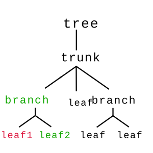
Example Tree Structure: The hierarchy remains central, but its selections are now compiled into stable index data before solver kernels run.
The methodological role of selection is therefore very specific. A selection is first a human-readable statement about a part of the model, for example one site, one spin sector, one boundary region, or one class of bonds. It is only after this selection is defined that it is resolved into stable integer data. This is the correct compromise between expressiveness and discipline. The framework remains physically legible, but numerical kernels still consume plain arrays, masks, and matrices.
The archival qttree.network lineage remains useful as a record of how the
original idea evolved, especially around broad Mapper-style tree slicing. But
it should now be treated as history rather than as the centre of the thesis
code. The layered package in qulab/core/qttree is the version that the thesis
is actually using.
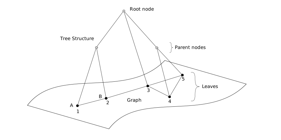
Tree structure remains the front-end language, but compilation resolves it into parent nodes, leaves, and graph relations that can be indexed explicitly in the numerical backend.
Basis, Support, Projectors, And Nambu Structure
The hierarchy is not only a software convenience; it is the way the theory chooses its one-particle basis. In the simplest tight-binding case the one-particle space is spanned by lattice sites and perhaps spin. In the thesis applications the basis is usually larger:
Here may mean a finite polytope, a strip, a periodic cell, a boundary region, or an island network. The orbital factor may be a real atomic-orbital model, an effective internal degree of freedom, or the sublattice structure of an SSH-type model. The spin factor may be present as an active magnetic degree of freedom or only as a degeneracy. QTTree’s role is to keep those labels visible until the model is deliberately compiled into a flat ordering.
This is also the right place to distinguish support from a projector. The support of an object says where it lives. A hopping term has bond support; an onsite potential has site support; a superconducting update has pairing-channel support; a boundary observable has edge or wall support. Support is therefore a statement about the domain of a term, field, update, or observable before it has become a numerical matrix.
A projector is a restriction or measurement on the already declared space. In the ideal mathematical language it is an operator with and . In the code it often appears as a sparse selector, mask, or compiled index list. A spin projector selects one spin channel; an orbital projector selects one internal component; an edge projector measures spectral weight near a boundary; a Nambu-sector projector separates particle-like and hole-like parts of a BdG eigenvector. The support says which physical region or channel exists; the projector says which part of the resulting basis or observable is being extracted.
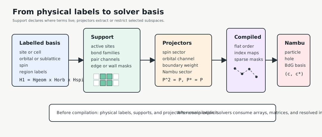
Figure 10.3: Basis, support, projector, and Nambu compilation pipeline.
The superconducting problems require one more conceptual step: Nambu doubling. After the ordinary one-particle basis has been chosen, a mean-field superconductor is represented in a doubled particle-hole space. With the convention
the quadratic Hamiltonian takes the BdG form
The precise sign and ordering conventions belong to the implementation and to the generalised BdG/SCMFT layer, but the methodological point is independent of those details. QTTree supplies the labelled basis, geometry, terms, support maps, and compilation boundary. The SCMFT layer then gives pairing fields, anomalous contractions, self-consistent updates, and free-energy accounting a superconducting interpretation.
Diagonalising the BdG matrix is the Bogoliubov transformation. The eigenvectors are decomposed into and components, and those components are the bridge from the numerical spectrum back to physical observables: density, magnetisation, anomalous density, LDOS, currents, channel amplitudes, and the mean-field free energy. Projectors and supports re-enter here because the observable is rarely the whole spectrum. The thesis usually asks for a projected statement: edge spectral weight, a wall-localised LDOS map, a pairing amplitude on a particular bond family, or the current circulating around a selected loop.
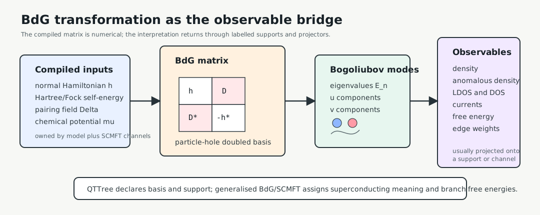
Figure 10.4: BdG transformation from compiled terms to projected observables.
Terms, Fields, And Rules
The second core idea is that geometry, Hamiltonian content, and self-consistency should remain distinct layers. A model should know what its sites and bonds are; it should know which terms are present in the Hamiltonian; and it should know which fields are externally imposed versus internally determined. These are related questions, but they are not the same question.
This matters especially for mean-field theory. In a weak implementation, one buries Hartree, Fock, or Gor’kov updates inside one solver that implicitly knows which entries of which array are supposed to be changed. In a stronger implementation, the channels and update rules are represented explicitly as part of the model description. That is the direction taken here. The framework does not treat self-consistency as an afterthought attached to a particular benchmark. It treats it as structured model data that can later be compiled into contractions, update maps, and solver steps.
That is also part of the conceptual contribution. The framework claims that mean-field theory should be expressed as a theory of channels, supports, and updates, not merely as an iterative numerical recipe. This makes the code more reproducible, but more importantly it makes the physics argument clearer.
Conceptually, this is why the code reads more like a language for Hamiltonians and fields than like a pile of chapter-specific numerical scripts. Terms say what is in the Hamiltonian. Fields say where order parameters or auxiliary quantities live. Interaction rules say how those fields should be updated or interpreted. Compilation and solving happen only after those distinctions have been made.
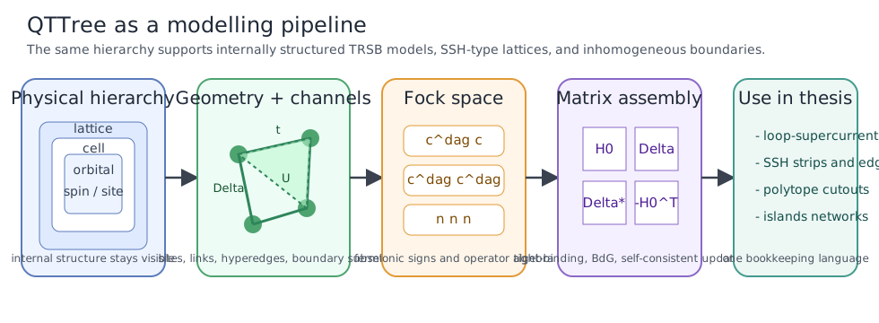
Figure 10.5 Hierarchy to Hamiltonian pipeline: The live pipeline is now hierarchy -> typed terms and fields -> compiled quadratic family -> solver result -> observable result.
Geometry As Data
The same separation appears in the treatment of geometry. A lattice is not merely a matrix dimension. It is a finite or periodic arrangement of repeated internal structure, together with optional masks, cutouts, and named regions. Open strips, impurity walls, SNS devices, and trimmed finite samples should therefore enter the framework as geometry data rather than as separate software branches.
This is one of the strongest practical gains of the current layered codebase. The topology line and the superconducting line no longer need different foundations just because one emphasises boundaries and the other emphasises self-consistency. Finite regions, polytopes, masks, and repeated unit cells can all be handled inside the same general geometry layer. The methodological point is simple: boundary conditions and spatial cutouts are part of the model, not special exceptions to it.
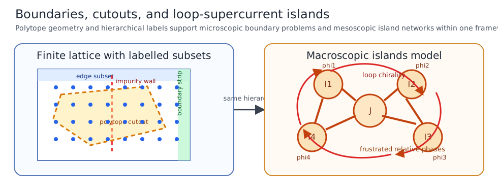
Finite geometries and islands networks: Polytope cutouts, labelled regions, and mesoscopic island devices are all treated as geometry data within the same lattice framework.
Compilation As A Boundary
The decisive architectural step in the live package is the explicit compilation layer between model specification and numerical solution. This is not just a software convenience. Methodologically it marks the point at which a physics description is turned into a solver-ready problem. Before compilation, the framework still speaks in terms of hierarchy, geometry, fields, and update rules. After compilation, it speaks in terms of resolved basis data, representations, and operator families.
That boundary is what allows one framework to cover both finite real-space and Bloch problems without pretending that they are numerically identical. They are different representations of the same modelling language. The compilation layer makes that distinction explicit, and the solver layer then consumes compiled problems rather than raw hierarchical objects. In other words, the code does not confuse expressiveness at the modelling level with cleverness at the numerical level.
This separation is one of the most conceptually important choices in the whole chapter. It says that the right response to numerical complexity is not to let numerical structures dominate the public language of the theory. Instead, one should make the translation from physical structure to numerical structure explicit and deliberate.
The final stage is the observable layer. This is where the framework becomes most clearly thesis-facing. The aim is not only to produce eigenvalues or convergence histories, but to produce structured physical statements: LDOS, QPI, pairing textures, current patterns, branch comparisons, effective free energies, overlap diagnostics, and topological markers. A result chapter should therefore be able to import a small number of benchmark or plotting wrappers, while the real physical post-processing lives in the common framework.
For self-consistent superconducting calculations, the decisive thesis object is not a single converged gap field but a branch decision. Uniform, staggered, winding, unitary, and nonunitary candidate states must be compared using the same channel convention and the same free-energy accounting. This is why the SCMFT layer exists as a separate owner rather than as a hidden option inside a generic QTT solver.
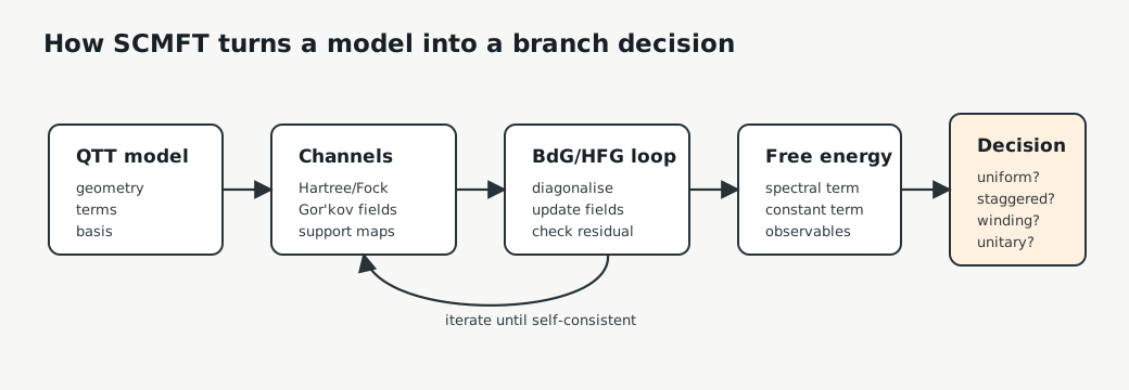
Figure 10.6: SCMFT branch-decision pipeline: model, channels, BdG/HFG iteration, free energy, and branch comparison.
Worked examples
Finite tight-binding and BdG kernels
The most mature finite real-space path is the square-lattice line used for the Friedel, impurity, and inhomogeneous BdG benchmarks. Conceptually its lesson is that a normal-state and a superconducting model can be treated as different specialisations of one common hierarchy-and-geometry framework. The same geometry can carry either ordinary hopping physics or mean-field superconducting physics, and the same solve-observe pattern then produces LDOS, QPI, and order parameter textures. This is exactly the sort of reuse that a thesis codebase should encourage.
Loop-supercurrent models
The loop-supercurrent branch uses the same hierarchy differently. There the important structure is not a large disordered lattice but a small internally structured unit cell, finite molecule, or island network whose sites carry phase-sensitive pairs and current channels. The same framework is therefore used to describe time-reversal-symmetric and time-reversal-breaking branches, not by introducing a second engine but by changing the model data and then solving the resulting compiled problem.
Just as importantly, the loop-supercurrent story is split into two logically different claims. The microscopic spacer model asks whether ordinary normal-mediated channels can make winding order win self-consistently. Its answer is limited and partly negative: winding can be diagnosed and sometimes enhanced, but the spectral stiffness and competing branches prevent it from becoming a clean material-realistic selection mechanism in the present model. The macroscopic island model is therefore not a redundant repeat. It is the controlled realisation layer that keeps the loop-current mechanism available while being honest about the microscopic model’s limitations.
Genetic and active search over device parameters
The Josephson-island work adds one more methodological layer: search over a large, structured model family. This is where the genetic algorithm belongs in the thesis. It is not a new solver and it is not part of the core QTT representation. It is a study-level search procedure built on top of the QTT/SCMFT pipeline.
The reason for using a genetic search is physical rather than decorative. The desired loop-supercurrent mechanism is narrow in parameter space. A winding branch is useful only when a competing nonwinding branch places anomalous density on a costly channel or sheet, and the winding phase can convert that antinode into a node. A rectangular grid wastes most of its evaluations on points where the relevant antinode is absent. The genetic search therefore uses cheap susceptibility and anomalous-density diagnostics to steer toward candidate geometries before any expensive nonlinear four-branch calculation is trusted.
There are two implemented versions of this idea. The microscopic
loop-supercurrent search is in
qulab/core/qttree/examples/studies/microscopic_loop_supercurrent/search/.
Its candidate object varies chemical potentials, attractive and repulsive
couplings, hopping amplitudes, and optional central/contact geometry flags.
The Josephson-island outer-sheet search is in
qulab/core/scmft/examples/mean_field/josephson_islands/search/outer_sheet_susceptibility_ga.py,
with the research-facing mirror in
qulab/research/ljc/islands/search/outer_sheet_susceptibility_ga.py.
That second search varies island and channel chemical potentials, island
attraction, repulsive sheet interactions, island separation, outer-strip
width, inner-sheet radius, corner rounding, contact geometry, and C4-compatible
boundary choices. The two paths share the same methodological role: generate
mechanism-aware candidates, not final phase-selection claims.
In code terms, a genome is a compact description of a Josephson-island device: island and channel chemical potentials, attractive and repulsive interaction strengths, island separation, strip width, contact geometry, inner-sheet radius, corner rounding, and C4-compatible boundary choices. The fitness function is deliberately mechanism-facing. It rewards winding-favouring linear response, survival of superconductivity on the islands, and antinodes that the winding branch can remove on outer or opposite-island loci. It penalises the inner-node and staggered-saving mechanisms, because those are precisely the competitors that can make a nonwinding branch win.
Schematically, the GA assigns a preselection score
where (x) is one proposed device genome. The favourable diagnostics (D_m)
include winding-favouring inverse susceptibility, outer-sheet or
opposite-island antinode weight, island anomalous-density survival, and
outer-over-inner selectivity. The competitor diagnostics (C_n) include
staggered outer saving, staggered inner saving, inner-node saving, excessive
spectral stiffness cost, and singular points whose apparent response is too
far from a controlled branch comparison. In the microscopic-loop implementation
this same logic appears as named terms such as outer_antinode_reward,
winding_outer_ados_saving_reward,
staggered_inner_ados_saving_penalty, spectral_cost_penalty, and, after
promotion, free_energy_advantage. In the Josephson-island implementation it
appears as the row score built from winding_node_minus_uniform_best,
outer_pi_node_saving_proxy, staggered_outer_pi_node_saving_proxy,
inner_pi_node_saving_proxy, and related response ratios. These names are
intentionally verbose: each score contribution is meant to be auditable in the
CSV output rather than hidden inside one black-box number.
The resulting workflow is:
- seed a population from prior scans and random admissible points;
- evaluate each point with inverse-susceptibility and ADOS-like diagnostics;
- rank the rows by a mechanism score;
- breed new candidates through elitism, crossover, mutation, and random injection;
- promote only the best candidates to full HFG branch comparison.
More explicitly, the population update used in the live code is an explore-exploit loop. The initial population is seeded partly from earlier CSV rows and partly from random admissible genomes. Duplicate candidates are filtered by a quantised key; for continuous profiles the key rounds controls to roughly three significant figures so that nearly identical proposals are not repeated. Elite candidates are copied forward. Children inherit each control from one of two parents, and then individual controls are mutated by either a discrete step on the allowed grid or by a bounded Gaussian step in continuous profiles. A fixed number of random new candidates is injected each generation to prevent the search from collapsing onto a single early pocket.
The cheap stage writes a full ledger rather than only the winner. For the
microscopic-loop search the default outputs are
microscopic_loop_genetic_susceptibility.csv and
microscopic_loop_genetic_followup.csv. For the Josephson-island search the
analogous outputs are named
josephson_island_outer_sheet_susceptibility_ga*.csv. These ledgers are part
of the method: they record which parameter values were proposed, which
diagnostic terms made them attractive, and which generation produced them.
This prevents the GA from being a hidden source of hand-selected examples.
This last step is the important methodological safeguard. A genetic-algorithm winner is only a proposal. It becomes thesis evidence only after the uniform, staggered, winding+, and winding- branches have been converged and compared with the same free-energy accounting and regional Hartree/Fock/Gor’kov decomposition. The GA therefore explains how promising island geometries were found; it does not define the physical branch-selection criterion.
The corresponding command-line entry points are deliberately small. A smoke run of the microscopic-loop search is
1PYTHONPATH=. python -m qulab.core.qttree.examples.studies.microscopic_loop_supercurrent.search.run_genetic_search --profile tinyand the island susceptibility search is
1PYTHONPATH=. python -m qulab.core.scmft.examples.mean_field.josephson_islands.search.outer_sheet_susceptibility_ga --profile tinyThe production runs used wider or focused profiles and more workers, but the tiny profiles are the regression-facing form: they prove that population generation, duplicate filtering, susceptibility evaluation, scoring, breeding, CSV checkpointing, and promotion hooks still work on a small problem.
The main physics lesson from the GA is also cautious. It helped find outer-node and central-node candidate mechanisms that would have been easy to miss in a rectangular scan. It did not by itself demonstrate a robust spontaneous winding ground state. In many promoted candidates, increasing the repulsive penalty also suppressed the anomalous density that the winding node was supposed to remove, or the spectral stiffness cost outweighed the local Gor’kov saving. This is exactly why the GA belongs in the methodology chapter: it is a principled way to search a difficult model family while keeping the final claim tied to self-consistent free energy rather than to an optimisation score.
Finite regions, SSH geometries, and topological Bloch models
The same framework also supports the thesis topology line. Weyl-SSH and Topo-BdG work require open boundaries, strips, masks, and momentum-space bulk descriptions. The important methodological point is that these are not treated as reasons to leave the framework. Instead, one changes the geometry or the representation while keeping the same general pipeline from model declaration to compiled problem to observable. In that sense the topology line is not a parallel framework branch, but another demanding use case of the same one.
That unification is itself part of the novelty. The thesis is not merely claiming that one package happens to cover several chapters. It is claiming that these chapters are best understood as different physical specialisations of one modelling grammar.
Scope and code lineage
The scope of the framework should therefore be stated precisely. QTTree is a physics-first modelling and Hamiltonian-compilation framework. Its strongest native path today is quadratic finite and Bloch modelling, together with self-consistent Hartree, Fock, and Gor’kov closures, finite-region geometry, and structured observables for the superconducting and topological lines of the thesis.
It is not, in its current thesis-facing form, best described as a generic
many-body operator-string engine with recursive Mapper logic at its centre.
Those ideas belong to the lineage recorded by the old qttree.network
monolith. They remain useful as archival context, but they should not dominate
the methodology chapter because they no longer describe the main public package
that the thesis is actually using.
This distinction matters. If the chapter overemphasises the old monolith, it undersells the genuinely stronger part of the current codebase: the layered split into labels, geometry, fields, interactions, compiled operator families, solvers, and observables. Conversely, if the chapter claims a full generic many-body framework, it overstates what the native package currently does best.
The correct methodological description is therefore not to revive the old interface in code, but to describe the live layered package honestly and use the old monolith only as lineage where that history clarifies design choices.
Conclusion
Quantum Tensor Tree provides a rigorous hierarchical description of
multicomponent quantum models, but the most important point is now architectural
rather than nostalgic. The live qulab/core/qttree package is a layered
framework in which labelled basis objects, typed terms and fields, compiled
quadratic families, numerically plain solvers, and structured observables form
one disciplined modelling pipeline. Together with qulab/core/scmft, that
includes not only LDOS, QPI, and topology observables, but also the
loop-supercurrent branch comparison, decomposition, active-search, and overlap
summaries that earlier thesis lineages treated more locally. The genetic
searches are part of that methodology only in this bounded sense: they are
mechanism-aware candidate generators whose outputs must still pass the same
self-consistent branch and free-energy tests as any hand-chosen parameter set.
That is the version of QTTree that should anchor the thesis. Its main value is conceptual: it gives the thesis one language for talking about structured quantum models across superconducting, loop-supercurrent, and topological applications, while making the passage from physical description to numerical representation explicit. It is rich enough to describe internally structured TRSB loop-supercurrent models, finite SNS and impurity geometries, and SSH or Topo-BdG boundary problems within one common framework, while remaining honest about where the current native surface is strongest.
References
- F. Bloch,
�Ber die quantenmechanik der elektronen in kristallgittern,
Zeitschrift f�r Physik, vol. 52, pp. 555–600, 1929. doi:10.1007/bf01339455 (↩︎) - C. Kittel, Introduction to solid state physics. Wiley, 2005. [Online]. Available: https://openlibrary.org/books/OL22152400M/Introduction_to_solid_state_physics (↩︎)
- J. Bardeen, L. Cooper, and J. Schrieffer,
Theory of superconductivity,
Phys. Rev., vol. 108, no. 5, pp. 1175–1204, 1957. doi:10.1103/PhysRev.108.1175 (↩︎) - L. Gor’kov,
Microscopic derivation of the ginzburg–landau equations in the theory of superconductivity,
Soviet Physics JETP, vol. 9, no. 6, pp. 1364–1367, 1959. (↩︎) - P. Gennes, Superconductivity of metals and alloys. Boca Raton: CRC Press, 2019. doi:10.1201/9780429497032 (↩︎)
- J. Hubbard,
Electron correlations in narrow energy bands,
Proceedings of the Royal Society of London. Series A. Mathematical and Physical Sciences, vol. 276, pp. 238–257, 1963. doi:10.1098/rspa.1963.0204 (↩︎) - R. Micnas, J. Ranninger, and S. Robaszkiewicz,
Superconductivity in narrow-band systems with local nonretarded attractive interactions,
Reviews of Modern Physics, vol. 62, pp. 113–171, 1990. doi:10.1103/revmodphys.62.113 (↩︎) - J. Kanamori,
Electron correlation and ferromagnetism of transition metals,
Progress of Theoretical Physics, vol. 30, pp. 275–289, 1963. doi:10.1143/ptp.30.275 (↩︎)